해당 자료는 전북대학교 이영미 교수님 2023고급시계열분석 자료임
############## package library (forecast) #ses library (data.table)library (ggplot2)library (lmtest) #dwtest library (TTR) #SMA library (lubridate)library (gridExtra)
Registered S3 method overwritten by 'quantmod':
  method            from
  as.zoo.data.frame zoo

Loading required package: zoo


Attaching package: ‘zoo’


The following objects are masked from ‘package:base’:

    as.Date, as.Date.numeric


Attaching package: ‘lubridate’


The following objects are masked from ‘package:data.table’:

    hour, isoweek, mday, minute, month, quarter, second, wday, week,
    yday, year


The following objects are masked from ‘package:base’:

    date, intersect, setdiff, union
1
# 데이터 불러오기 <- scan ("mindex.txt" )
\(S_n^{(1)} = w \sum_{j=0}^{n-1} (1-w)^j Z_{n-j} + (1-w)^n S_0^{(1)}\)
<- function (z,w,s0){<- c ()1 ] <- w* z[1 ] + (1 - w)* s0for (k in 2 : length (z)){<- w * z[k] + (1 - w)* Sn[k-1 ]return (Sn)
.6 <- simple_exp_smoothing (z,0.6 ,15 ).2 <- simple_exp_smoothing (z,0.2 ,15 )
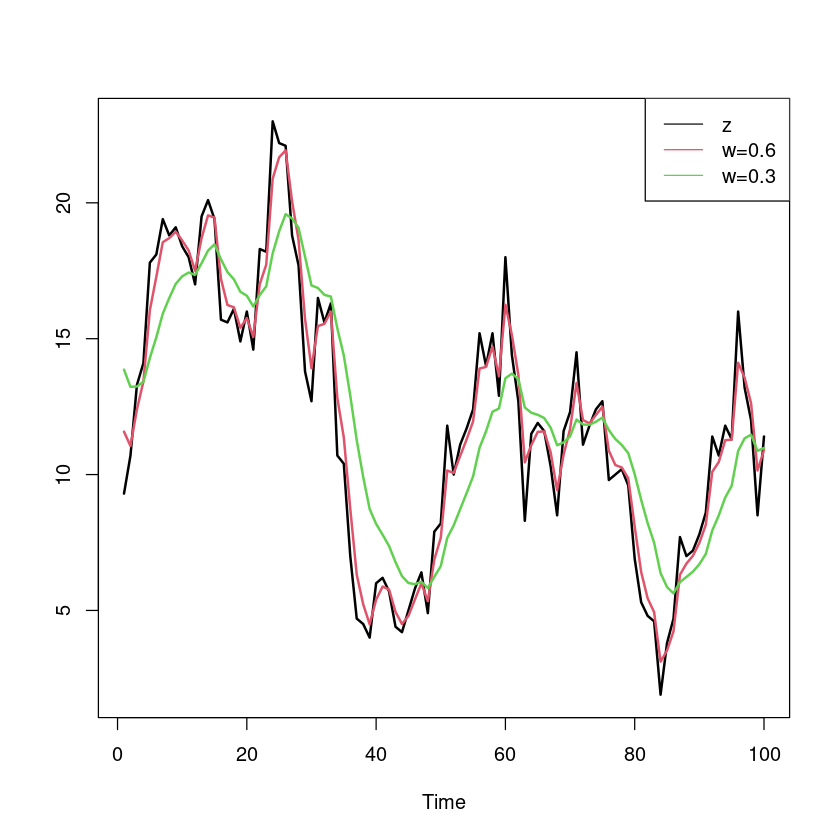
ts.plot (ts (z), ses_0.6 , ses_0.2 , col= 1 : 3 , lwd= 2 )legend ("topright" , legend = c ("z" ,"w=0.6" ,"w=0.3" ), col= 1 : 3 , lty= 1 )
W값이 클수록 원 데이터와 비슷하고, 평활 효과가 작아진다.
W값이 작을수록 원데이터를 천천히 따라가고, 평활 효과가 커진다.
\(\hat Z_{t-1}(1) = S_{t-1}^{(1)}\) 이므로
<- c (2 ,3 ,99 ,100 ).6 [point-1 ].2 [point-1 ]
11.58 11.052 12.6262842848221 10.1505137139288
13.86 13.228 11.4677321254815 10.8741857003852
2
(1)
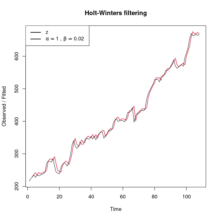
추세가 있기 때문에 이중지수평활법을 사용한다.
<- HoltWinters (z, gamma = FALSE )
Holt-Winters exponential smoothing with trend and without seasonal component.

Call:
HoltWinters(x = z, gamma = FALSE)

Smoothing parameters:
 alpha: 1
 beta : 0.01666631
 gamma: FALSE

Coefficients:
        [,1]
a 667.000000
b   5.145043
plot (female_smoothing, lwd= 2 )legend ("topleft" , legend= c ("z" ,expression (alpha == 1 ~ "," ~ beta== 0.02 )), lty= 1 , lwd= 2 )
- 예측오차 분석
head (female_smoothing$ fitted)
A Time Series: 6 × 3
3
230.0000
223
7.000000
4
235.9833
229
6.983334
5
241.9669
235
6.966945
6
233.7175
227
6.717501
7
242.7555
236
6.755542
8
238.5763
232
6.576287
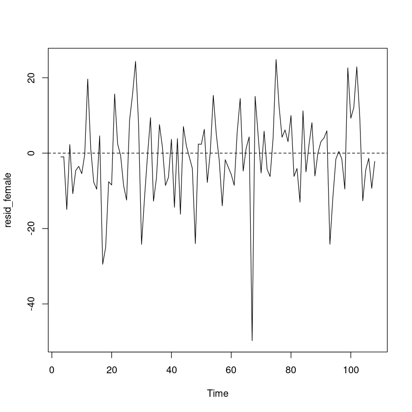
HoltWinters 함수를 사용하는 경우, 이중지수 평활값이 3번째부터 구해진다. 따라서 예측오차 역시 원데이터의 3번째 값부터 구할 수 있다.
<- z[- (1 : 2 )] - female_smoothing$ fitted[,1 ] #또는 <- resid (female_smoothing) #같은 방법임
plot.ts (resid_female)abline (h= 0 , lty= 2 )
예측오차의 경우 0을 중심으로 대칭이고, 이분산성은 없어 보인다.
    One Sample t-test

data:  resid_female
t = -0.93497, df = 105, p-value = 0.3519
alternative hypothesis: true mean is not equal to 0
95 percent confidence interval:
 -3.276746  1.176749
sample estimates:
mean of x
-1.049998
t-test 결과 예측오차의 평균은 0이라고 할 수 있다.
:: dwtest (lm (resid_female~ 1 ), alternative= "two.sided" )
    Durbin-Watson test

data:  lm(resid_female ~ 1)
DW = 1.7861, p-value = 0.2662
alternative hypothesis: true autocorrelation is not 0
(2)
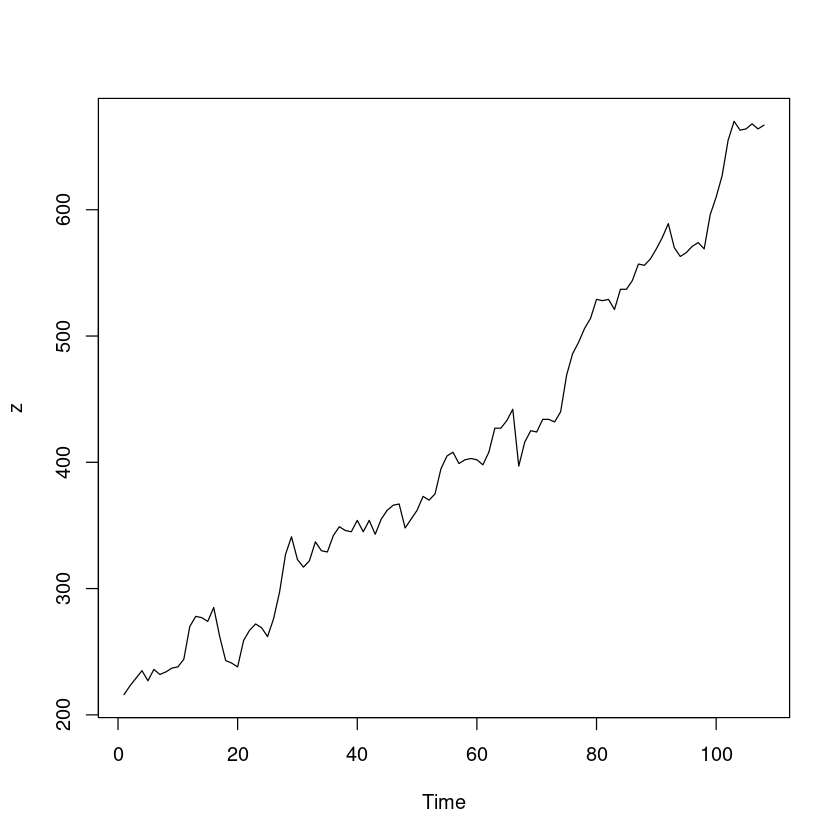
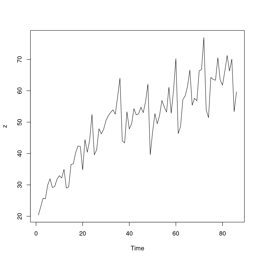
<- scan ("export.txt" )plot.ts (z)
지난 과제에 언급한대로 이 시계열에는 이분산성은 없다고 할 수 있다.
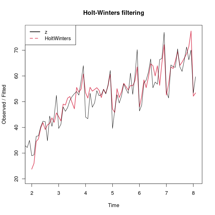
추세와 계절성분이 있으므로 계절주기가 12, 가법형 계절평활법을 사용하는 것이 적합하다.
계절평활을 하기 위해서는 데이터를 ts 객체로 변환해야 한다
<- ts (z, frequency= 12 )
<- HoltWinters (z_ts)
Holt-Winters exponential smoothing with trend and additive seasonal component.

Call:
HoltWinters(x = z_ts)

Smoothing parameters:
 alpha: 0.3304767
 beta : 0.04369053
 gamma: 0.6102758

Coefficients:
           [,1]
a    66.9300146
b     0.3670945
s1   -0.9590061
s2   -2.3460160
s3   -1.4388022
s4    4.0020957
s5   -2.8546787
s6   -3.1036803
s7    0.4486017
s8    3.3118493
s9    1.6302355
s10   8.0731659
s11 -11.5480012
s12  -8.8892298
plot (export_smoothing, lwd= 2 , lty= 1 : 2 )legend ("topleft" , legend= c ("z" , "HoltWinters" ), col= 1 : 2 , lty= 1 : 2 , lwd= 2 )
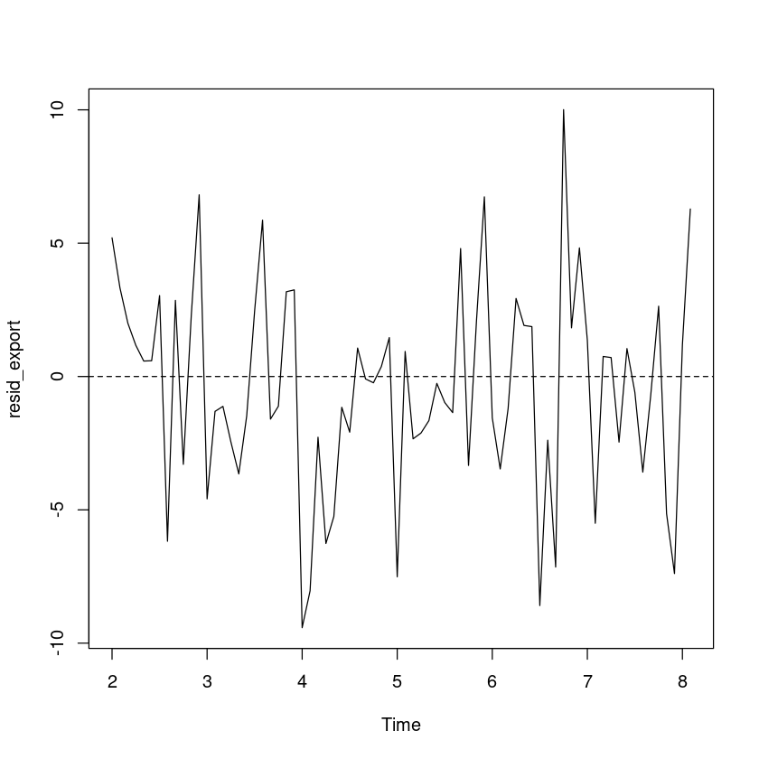
- 예측오차분석
<- resid (export_smoothing)plot.ts (resid_export)abline (h= 0 , lty= 2 )
예측오차의 경우 0을 중심으로 대칭이고, 이분산성은 없어 보인다
    One Sample t-test

data:  resid_export
t = -0.99304, df = 73, p-value = 0.324
alternative hypothesis: true mean is not equal to 0
95 percent confidence interval:
 -1.359825  0.455374
sample estimates:
 mean of x
-0.4522256
t-test 결과 예측오차의 평균은 0이라고 할 수 있다.
:: dwtest (lm (resid_export~ 1 ), alternative= "two.sided" )
    Durbin-Watson test

data:  lm(resid_export ~ 1)
DW = 1.8163, p-value = 0.4267
alternative hypothesis: true autocorrelation is not 0
DW test 결과 예측오차들 간의 자기 상관은 없는 것으로 보인다.
따라서 예측오차는 분석 결과 평활 결과는 적합하다고 할 수 있다.
2장에서 계절추세 모형을 적합한 경우에는 예측오차 간에 자기 상관이 있다는 결과 를 얻었었는데, 평활을 이용한 결과 자기상관이 제거되었다.
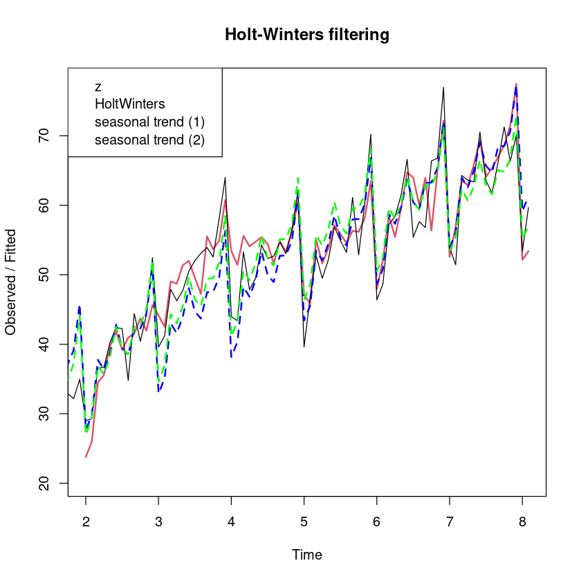
- 계절추세모형
<- as.factor (cycle (z_ts))<- 1 : length (z)<- lm (z~ t+ seasonal_I)<- lm (z~ t+ I (t^ 2 )+ seasonal_I)
plot (export_smoothing, lwd= 2 , lty= 1 : 2 )lines (ts (fitted (m2), frequency= 12 ), col= 'blue' , lty= 2 , lwd= 2 )lines (ts (fitted (m3), frequency= 12 ), col= 'green' , lty= 2 , lwd= 2 )legend ("topleft" , legend= c ("z" , "HoltWinters" , "seasonal trend (1)" , "seasonal trend (2)" ))
- SSE 비교하기
head (export_smoothing$ fitted) ## 평활값은 12시차 이후값부터 생성됨
A Time Series: 6 × 4
Jan 2
23.77825
28.21682
0.8502812
-5.2888542
Feb 2
25.99728
30.78616
0.9253878
-5.7142708
Mar 2
34.53331
32.80963
0.9733636
0.7503125
Apr 2
35.55911
34.44285
1.0021933
0.1140625
May 2
39.71058
35.83200
1.0190994
2.8594792
Jun 2
41.81786
37.04258
1.0274655
3.7478125
<- sum ((z[- (1 : 12 )]- export_smoothing$ fitted[,1 ])^ 2 ) #또는 <- export_smoothing$ SSE
<- sum (resid (m2)^ 2 )<- sum (resid (m3)^ 2 )
paste0 ("SSE_smomthing = " ,sse_smoothing)paste0 ("SSE_m2 = " , sse_m2)paste0 ("SSE_m3 = " , sse_m3)
'SSE_smomthing = 1135.42182593918'
'SSE_m2 = 1371.05731181319'
'SSE_m3 = 934.603221419272'
모형을 1시차 예측오차에 대한 제곱합으로 비교하면 2차추세모형을 적합한 m3의 SSE값이 가장 작고, 1차선형추세를 사용한 모형의 SSE가 가장 크다.
<- mean ((z[- (1 : 12 )]- export_smoothing$ fitted[,1 ])^ 2 )<- mean (resid (m2)^ 2 )<- mean (resid (m3)^ 2 )paste0 ("MSE_smomthing = " ,mse_smoothing)paste0 ("MSE_m2 = " , mse_m2)paste0 ("MSE_m3 = " , mse_m3)
'MSE_smomthing = 15.3435381883673'
'MSE_m2 = 15.9425268815487'
'MSE_m3 = 10.8674793188287'
3
(1)
<- read.csv ('data1.csv' )head (dt)
A data.frame: 6 × 3
<int>
<int>
<dbl>
1
1
1
-1.5346871
2
2
2
2.6850469
3
3
3
-0.4288189
4
4
4
1.3724199
5
5
5
-0.9800884
6
6
6
2.4156505
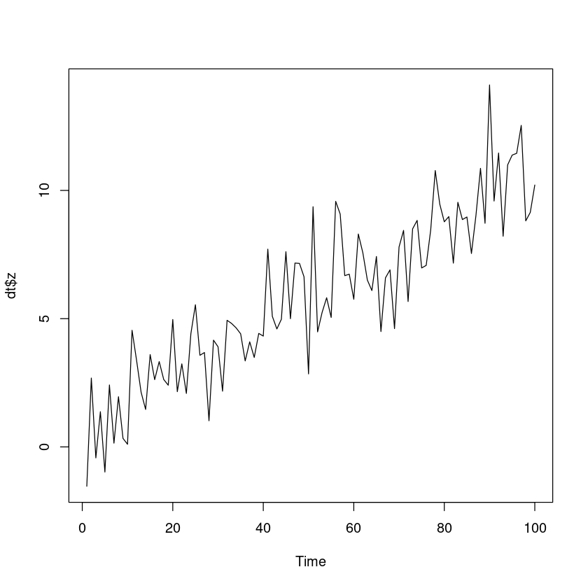
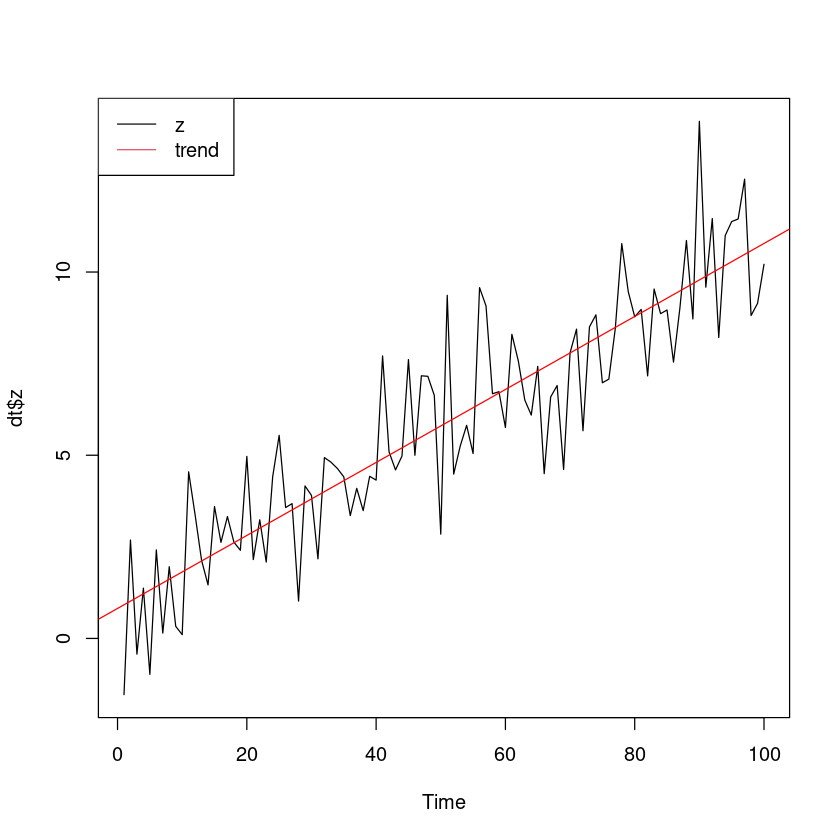
추세가 있음, 계절성분은 없음
선형추세 모형 적합
<- lm (z~ t, dt)summary (m_trend)
Call:
lm(formula = z ~ t, data = dt)

Residuals:
    Min      1Q  Median      3Q     Max
-3.0803 -1.0287  0.0169  0.8426  4.3288

Coefficients:
            Estimate Std. Error t value Pr(>|t|)
(Intercept) 0.818932   0.296301   2.764  0.00682 **
t           0.099619   0.005094  19.557  < 2e-16 ***
---
Signif. codes:  0 ‘***’ 0.001 ‘**’ 0.01 ‘*’ 0.05 ‘.’ 0.1 ‘ ’ 1

Residual standard error: 1.47 on 98 degrees of freedom
Multiple R-squared:  0.796, Adjusted R-squared:  0.7939
F-statistic: 382.5 on 1 and 98 DF,  p-value: < 2.2e-16
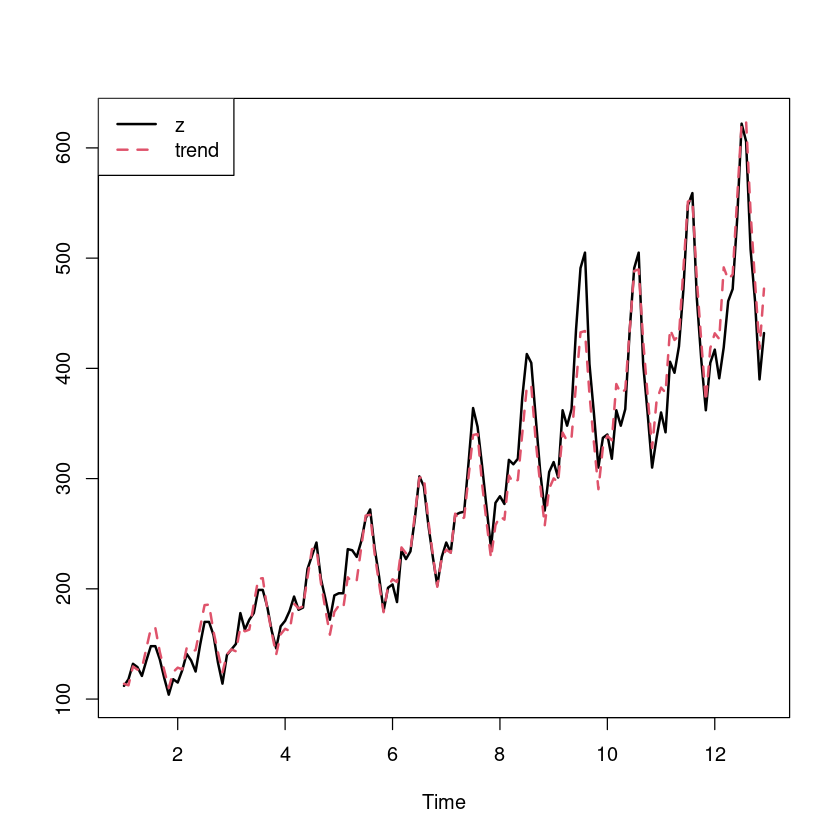
plot.ts (dt$ z)abline (m_trend, col= 'red' )legend ("topleft" , c ("z" , "trend" ), lty= 1 , col= 1 : 2 )
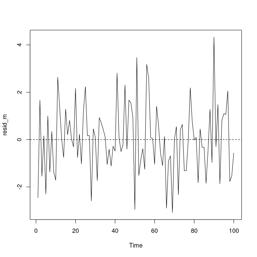
- 잔차분석
<- resid (m_trend)plot.ts (resid_m)abline (h= 0 , lty= 2 )
잔차의 경우 0을 중심으로 대칭이고, 이분산성은 없어 보인다.
    One Sample t-test

data:  resid_m
t = -5.2362e-16, df = 99, p-value = 1
alternative hypothesis: true mean is not equal to 0
95 percent confidence interval:
 -0.2902834  0.2902834
sample estimates:
    mean of x
-7.660376e-17
t-test 결과 예측오차의 평균은 0이라고 할 수 있다
    Durbin-Watson test

data:  m_trend
DW = 2.2164, p-value = 0.8389
alternative hypothesis: true autocorrelation is greater than 0
(2)
<- data.frame (t= 100 + (1 : 10 ))<- predict (m_trend, new_dt)
1 10.8804416292757 2 10.9800605357706 3 11.0796794422655 4 11.1792983487603 5 11.2789172552552 6 11.3785361617501 7 11.4781550682449 8 11.5777739747398 9 11.6773928812347 10 11.7770117877295
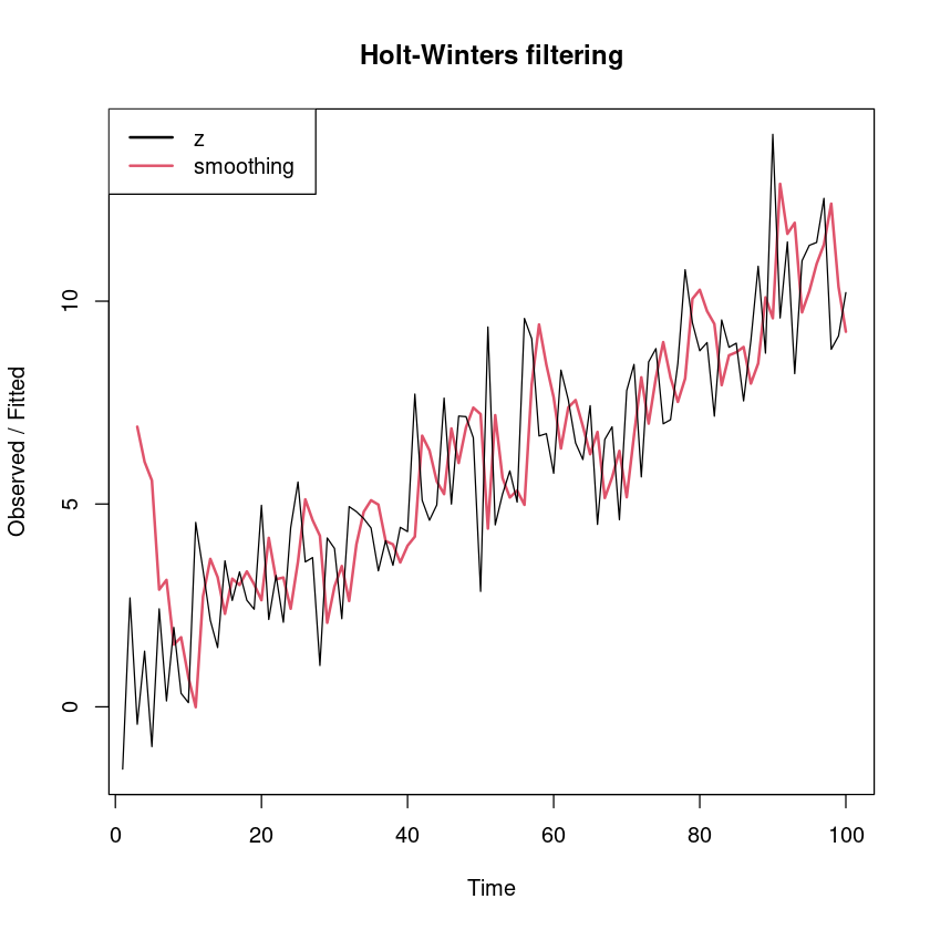
(3)
<- HoltWinters (dt$ z, gamma= FALSE )
Holt-Winters exponential smoothing with trend and without seasonal component.

Call:
HoltWinters(x = dt$z, gamma = FALSE)

Smoothing parameters:
 alpha: 0.496601
 beta : 0.396225
 gamma: FALSE

Coefficients:
        [,1]
a  9.7266353
b -0.3150449
plot (m_smoothing, lwd= 2 )legend ("topleft" , legend= c ("z" ,"smoothing" ), lty= 1 , lwd= 2 , col= 1 : 2 )
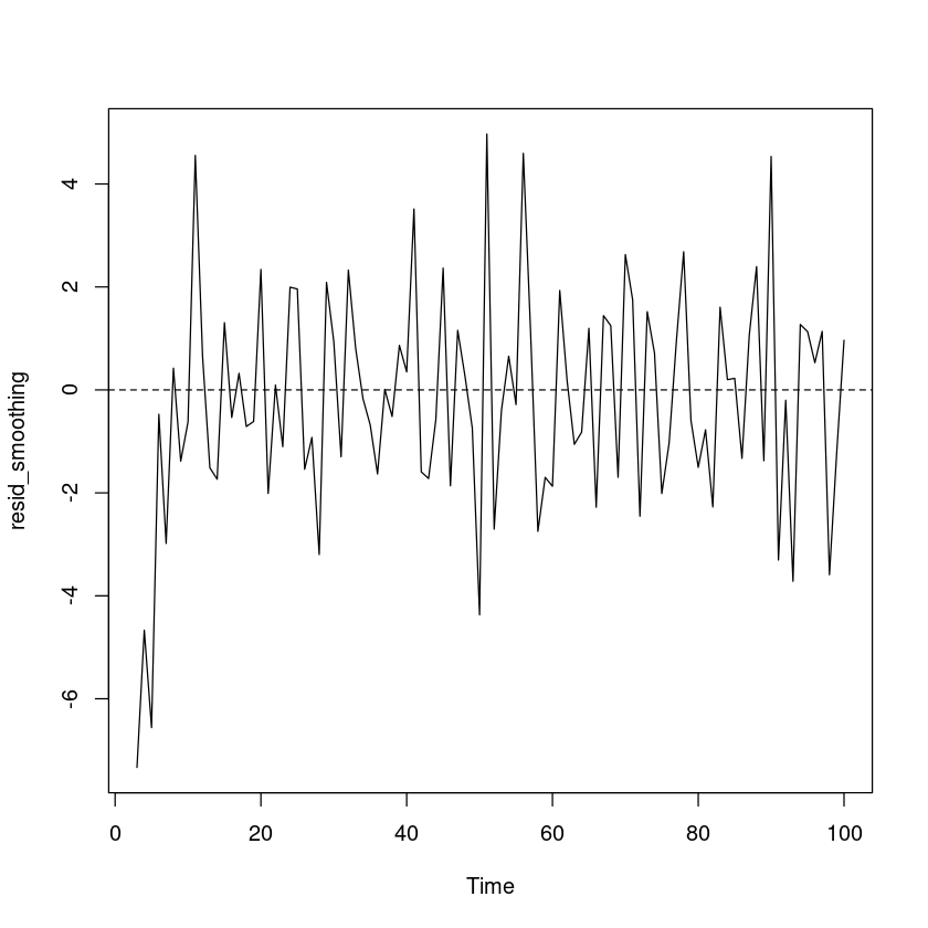
- 예측오차 분석
<- dt$ z[- (1 : 2 )] - m_smoothing$ fitted[,1 ] #또는 <- resid (m_smoothing) #같은 방법임
plot.ts (resid_smoothing)abline (h= 0 , lty= 2 )
예측오차의 경우 0을 중심으로 대칭이고, 이분산성은 없어 보인다.
    One Sample t-test

data:  resid_smoothing
t = -1.0711, df = 97, p-value = 0.2868
alternative hypothesis: true mean is not equal to 0
95 percent confidence interval:
 -0.6709125  0.2005740
sample estimates:
 mean of x
-0.2351693
t-test 결과 예측오차의 평균은 0이라고 할 수 있다.
:: dwtest (lm (resid_smoothing~ 1 ), alternative= "two.sided" )
    Durbin-Watson test

data:  lm(resid_smoothing ~ 1)
DW = 1.9664, p-value = 0.8675
alternative hypothesis: true autocorrelation is not 0
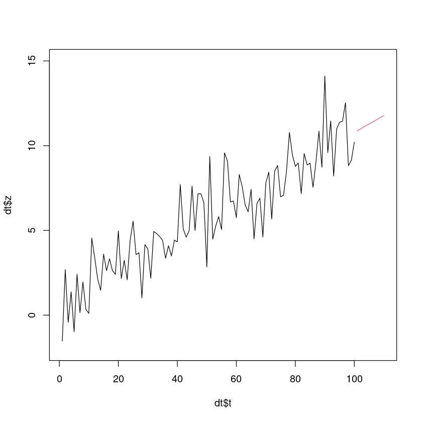
(4)
<- predict (m_smoothing, n.ahead= 10 , prediction.interval = T, level= 0.95 )
A Time Series: 10 × 3
101
9.411590
13.67142
5.1517644
102
9.096545
14.28017
3.9129175
103
8.781500
15.20395
2.3590541
104
8.466456
16.38382
0.5490889
105
8.151411
17.77356
-1.4707380
106
7.836366
19.34098
-3.6682458
107
7.521321
21.06388
-6.0212357
108
7.206276
22.92649
-8.5139377
109
6.891231
24.91716
-11.1346959
110
6.576186
27.02692
-13.8745530
:: holt (dt$ z, alpha = m_smoothing$ alpha, beta= m_smoothing$ beta, h= 10 )#, initial)
    Point Forecast       Lo 80    Hi 80      Lo 95    Hi 95
101       8.862685   6.0523463 11.67302   4.564643 13.16073
102       8.360702   4.5932352 12.12817   2.598859 14.12254
103       7.858719   2.6320999 13.08534  -0.134705 15.85214
104       7.356735   0.3034311 14.41004  -3.430363 18.14383
105       6.854752  -2.3086731 16.01818  -7.159497 20.86900
106       6.352769  -5.1561498 17.86169 -11.248603 23.95414
107       5.850786  -8.2094249 19.91100 -15.652451 27.35402
108       5.348803 -11.4485541 22.14616 -20.340538 31.03814
109       4.846819 -14.8590196 24.55266 -25.290661 34.98430
110       4.344836 -18.4296256 27.11930 -30.485697 39.17537
잘려서 뒤에가 뭐라고 써있는지를 모르겠음. initial값에 뭘 지정하는 것 같은데 똑같은 값이 안나온다
(5)
<- read.csv ("data1_new.csv" )
A data.frame: 10 × 3
<int>
<int>
<dbl>
1
101
11.577471
2
102
13.171004
3
103
12.730258
4
104
12.242375
5
105
10.877077
6
106
13.297355
7
107
14.632224
8
108
15.049088
9
109
9.671734
10
110
12.216420
plot (dt$ t,dt$ z, xlim= c (1 ,110 ), ylim= c (- 2 , 15 ), type= 'l' )lines (101 : 110 , pred_trend, col= 2 )lines (101 : 110 , pred_smoothing, col= 3 )
ERROR: Error in xy.coords(x, y): 'x' and 'y' lengths differ
MSE, MAPE, MAE 값을 이용하여 비교할 수 있다.
\(MSE = \dfrac{1}{m} \sum_{i=1}^n \hat e_{n-1+t}(1)^2\)
\(MAPE = \dfrac{100}{n} \sum_{i=1}^n \left| \dfrac{\hat e_{n-1+t}(1)}{Z_{n+t}} \right|\)
\(MAE = \dfrac{1}{m} \sum_{i=1}^m \left| \hat e_{n-1+t}(1) \right|\)
<- real_new_dt$ z - pred_trend<- real_new_dt$ z - pred_smoothing
MSE_trend = mean (e_trend^ 2 ))MSE_smoothing = mean (e_smoothing^ 2 ))MAPE_trend = 100 * sum (abs (e_trend/ real_new_dt$ z)) / 10 )MAPE_smoothing = 100 * sum (abs (e_smoothing/ real_new_dt$ z)) / 10 )MAE_trend = mean (abs (e_trend)))MAE_smoothing = mean (abs (e_smoothing)))
3.91978903404576
127.173436899506
13.1385437579375
218.735568237967
1.69927387507187
9.02750167882282
교수님 풀이랑 smoothing 의 값이 좀 다르다.
4
<- scan ('export.txt' )plot.ts (z)
(1)
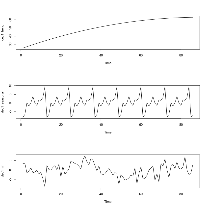
위에서 2차선형추세 모형이 더 적절했다고 했으므로, 2차 추세 모형을 적합한다.
<- ts (z, frequency= 12 )<- as.factor (cycle (z_ts))<- 1 : length (z)
<- fitted (lm (z~ t+ I (t^ 2 ))) ## 추세성분
= z- dec1_trend<- fitted (lm (adjtrend ~ 0 + seasonal_I)) ## 계절성분
= z- dec1_trend- dec1_seasonal ## 불규칙 성분
par (mfrow= c (3 ,1 ))plot.ts (dec1_trend)plot.ts (dec1_seasonal)plot.ts (dec1_irr)abline (h= 0 , lty= 2 )= c (1 ,1 )
(2)
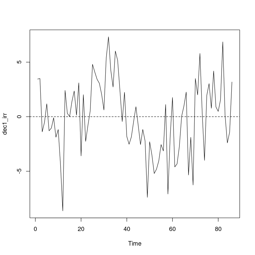
plot.ts (dec1_irr)abline (h= 0 , lty= 2 )
예측오차의 경우 0을 중심으로 대칭이고, 이분산성은 보이지 않는다.
    One Sample t-test

data:  dec1_irr
t = 2.2831e-16, df = 85, p-value = 1
alternative hypothesis: true mean is not equal to 0
95 percent confidence interval:
 -0.7179805  0.7179805
sample estimates:
   mean of x
8.244475e-17
t-test 결과 예측오차의 평균은 0이라고 할 수 있다.
:: dwtest (lm (dec1_irr~ 1 ), alternative= "two.sided" )
    Durbin-Watson test

data:  lm(dec1_irr ~ 1)
DW = 1.1429, p-value = 2.78e-05
alternative hypothesis: true autocorrelation is not 0
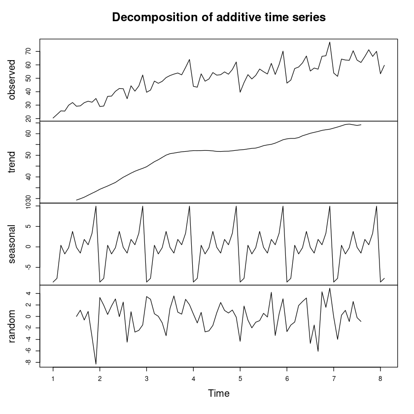
(3)
<- decompose (z_ts, 'additive' )plot (dec_fit)
(4)
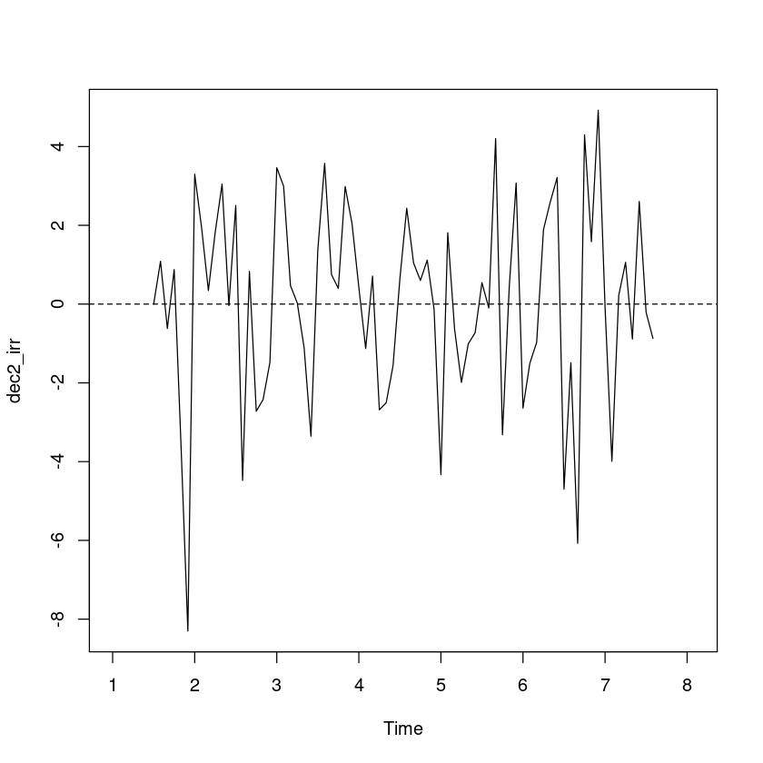
<- dec_fit$ randomplot.ts (dec2_irr)abline (h= 0 , lty= 2 )
예측오차의 경우 0을 중심으로 대칭이고, 이분산성은 없어 보인다.
    One Sample t-test

data:  dec2_irr
t = 0.074013, df = 73, p-value = 0.9412
alternative hypothesis: true mean is not equal to 0
95 percent confidence interval:
 -0.5674456  0.6112171
sample estimates:
 mean of x
0.02188575
t-test 결과 예측오차의 평균은 0이라고 할 수 있다
:: dwtest (lm (dec2_irr~ 1 ), alternative= "two.sided" )
    Durbin-Watson test

data:  lm(dec2_irr ~ 1)
DW = 1.9469, p-value = 0.8188
alternative hypothesis: true autocorrelation is not 0
DW test 결과 예측오차들 간의 자기 상관은 없는 것으로 보인다.
따라서 예측오차는 분석 결과 평활 결과는 적절하다고 할 수 있다.
추세를 이용한 분해법에서 예측 오차는 상관관계가 있었지만, 평활법을 사용하면서 예측오차들의 상관관계를 제거할 수 있었다.
(5)
= sum (dec1_irr^ 2 )= sum (dec2_irr^ 2 , na.rm= T)paste0 ("SSE_1 = " , sse_1)paste0 ("SSE_2 = " , sse_2)
'SSE_1 = 953.219486362055'
'SSE_2 = 472.381499188028'
SSE 값을 비교하였을 때, 평활에 의한 분해법의 값이 더 작다.
= mean (dec1_irr^ 2 )= mean (dec2_irr^ 2 , na.rm= T)paste0 ("MSE_1 = " , mse_1)paste0 ("MSE_2 = " , mse_2)
'MSE_1 = 11.0839475158378'
'MSE_2 = 6.38353377281119'
5
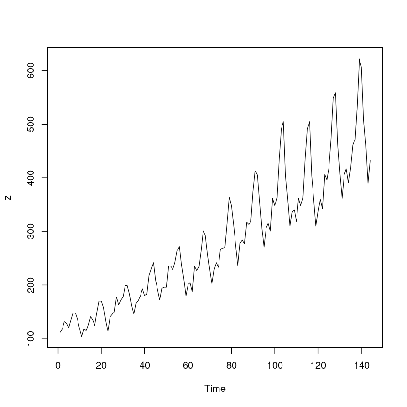
<- scan ('usapass.txt' )plot.ts (z)
(1)
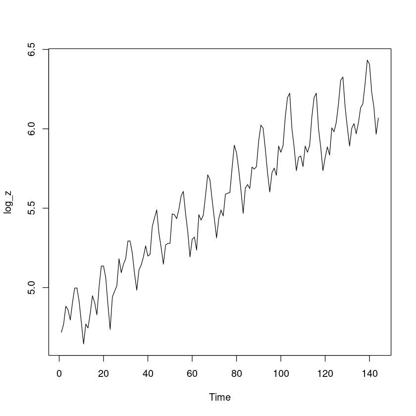
<- log (z)plot.ts (log_z)
(2)
지수함수를 사용한 계절형 추세모형을 적합한다.
<- ts (z, frequency= 12 )= log (z_ts)<- as.factor (cycle (log_z_ts))<- 1 : length (z)<- lm (log_z_ts~ 0 + t+ seasonal_I)summary (m_trend)
Call:
lm(formula = log_z_ts ~ 0 + t + seasonal_I)

Residuals:
      Min        1Q    Median        3Q       Max
-0.159814 -0.044426  0.000623  0.045572  0.151846

Coefficients:
              Estimate Std. Error t value Pr(>|t|)
t            0.0100999  0.0001252   80.67   <2e-16 ***
seasonal_I1  4.7246982  0.0198289  238.27   <2e-16 ***
seasonal_I2  4.7026123  0.0198822  236.52   <2e-16 ***
seasonal_I3  4.8342011  0.0199361  242.49   <2e-16 ***
seasonal_I4  4.8015084  0.0199907  240.19   <2e-16 ***
seasonal_I5  4.8009618  0.0200459  239.50   <2e-16 ***
seasonal_I6  4.9237482  0.0201017  244.94   <2e-16 ***
seasonal_I7  5.0296649  0.0201582  249.51   <2e-16 ***
seasonal_I8  5.0223242  0.0202153  248.44   <2e-16 ***
seasonal_I9  4.8708171  0.0202729  240.26   <2e-16 ***
seasonal_I10 4.7357833  0.0203312  232.93   <2e-16 ***
seasonal_I11 4.5905564  0.0203901  225.14   <2e-16 ***
seasonal_I12 4.7032829  0.0204496  229.99   <2e-16 ***
---
Signif. codes:  0 ‘***’ 0.001 ‘**’ 0.01 ‘*’ 0.05 ‘.’ 0.1 ‘ ’ 1

Residual standard error: 0.06224 on 131 degrees of freedom
Multiple R-squared:  0.9999,    Adjusted R-squared:  0.9999
F-statistic: 8.844e+04 on 13 and 131 DF,  p-value: < 2.2e-16
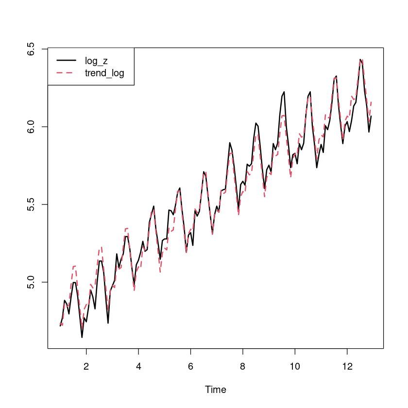
\(\hat Z_t = 0.01t + 4.72I_1 + 4.70I_2 + \dots + 4.70I_{12}\)
ts.plot (log_z_ts, ts (fitted (m_trend), frequency= 12 ), col= 1 : 2 , lty= 1 : 2 , lwd= 2 )legend ("topleft" , c ("log_z" , "trend_log" ), col= 1 : 2 , lty= 1 : 2 , lwd= 2 )
ts.plot (z_ts, ts (exp (fitted (m_trend)), frequency= 12 ), col= 1 : 2 , lty= 1 : 2 , lwd= 2 )legend ("topleft" , c ("z" , "trend" ), col= 1 : 2 , lty= 1 : 2 , lwd= 2 )
- 잔차분석
<- resid (m_trend)plot.ts (resid_m)abline (h= 0 , lty= 2 )
잔차의 경우 0을 중심으로 대칭이고, 이분산성은 없어 보인다
    One Sample t-test

data:  resid_m
t = -5.2362e-16, df = 99, p-value = 1
alternative hypothesis: true mean is not equal to 0
95 percent confidence interval:
 -0.2902834  0.2902834
sample estimates:
    mean of x
-7.660376e-17
t-test 결과 예측오차의 평균은 0이라고 할 수 있다.
:: dwtest (m_trend, alternative= "two.sided" )
    Durbin-Watson test

data:  m_trend
DW = 0.40831, p-value < 2.2e-16
alternative hypothesis: true autocorrelation is not 0
(3)
- 로그변환한 데이터에 대한 가법 모형
<- HoltWinters (log_z_ts)
Holt-Winters exponential smoothing with trend and additive seasonal component.

Call:
HoltWinters(x = log_z_ts)

Smoothing parameters:
 alpha: 0.3447498
 beta : 0.003585913
 gamma: 0.879488

Coefficients:
            [,1]
a    6.165298459
b    0.008744433
s1  -0.073696849
s2  -0.142822821
s3  -0.039964334
s4   0.015968620
s5   0.033673237
s6   0.157016140
s7   0.300626468
s8   0.285698068
s9   0.098491289
s10 -0.021898771
s11 -0.190036243
s12 -0.096734648
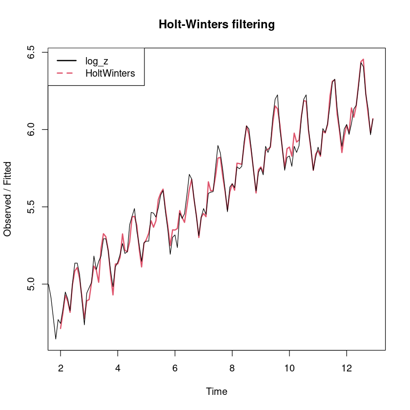
plot (m_smoothing, lwd= 2 , lty= 1 : 2 )legend ("topleft" , legend= c ("log_z" , "HoltWinters" ), col= 1 : 2 , lty= 1 : 2 , lwd= 2 )
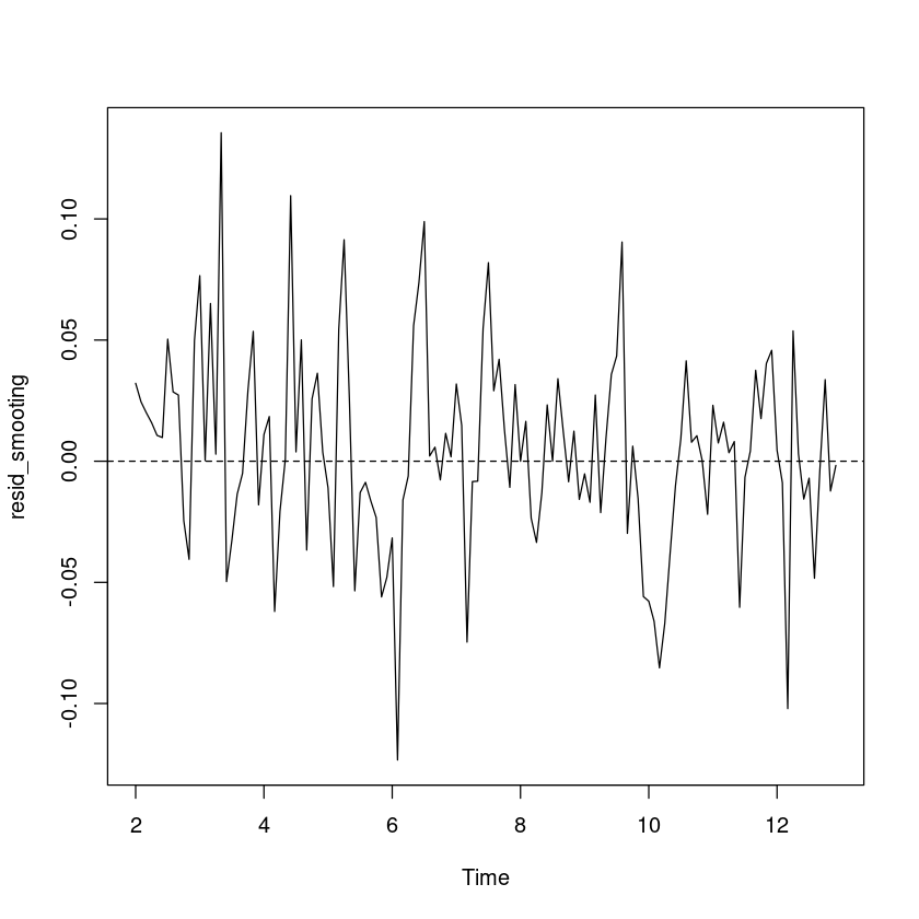
- 잔차분석
<- resid (m_smoothing)plot.ts (resid_smooting)abline (h= 0 , lty= 2 )
예측오차의 경우 0을 중심으로 대칭이고, 이분산성은 없어 보인다.
    One Sample t-test

data:  resid_smooting
t = 1.2026, df = 131, p-value = 0.2313
alternative hypothesis: true mean is not equal to 0
95 percent confidence interval:
 -0.002766709  0.011346227
sample estimates:
  mean of x
0.004289759
t-test 결과 예측오차의 평균은 0이라고 할 수 있다.
:: dwtest (lm (resid_smooting~ 1 ), alternative= "two.sided" )
    Durbin-Watson test

data:  lm(resid_smooting ~ 1)
DW = 1.4549, p-value = 0.001604
alternative hypothesis: true autocorrelation is not 0
DW test 결과 예측오차들 간의 자기 상관이 있는 것으로 보인다.
하지만, 추세모형을 적합하였을 때 얻어진 잔차에 비해 유의확률값이 크다.
예측오차는 분석 결과 추세모형 적합 결과보다는 평활 결과가 더 적절하다고 할 수 있다.
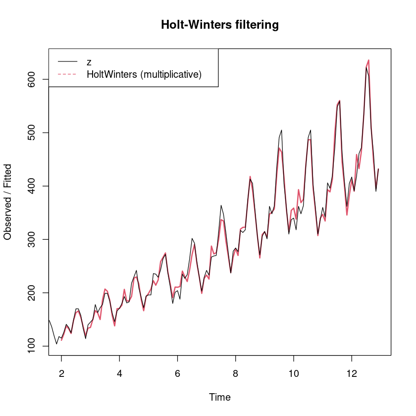
- 원 데이터에 대한 승법모형 적용
<- HoltWinters (z_ts, seasonal = "multiplicative" )
Holt-Winters exponential smoothing with trend and multiplicative seasonal component.

Call:
HoltWinters(x = z_ts, seasonal = "multiplicative")

Smoothing parameters:
 alpha: 0.3204565
 beta : 0.02388265
 gamma: 1

Coefficients:
           [,1]
a   464.9721064
b     2.7859138
s1    0.9464640
s2    0.8810274
s3    0.9648716
s4    1.0334898
s5    1.0470250
s6    1.1793118
s7    1.3631491
s8    1.3399425
s9    1.1195987
s10   0.9993794
s11   0.8438225
s12   0.9290880
plot (m_smoothing_multi, lwd= 2 , lty= 1 : 2 )legend ("topleft" , legend= c ("z" , "HoltWinters (multiplicative)" ), col= 1 : 2 , lty= 1 : 2 )
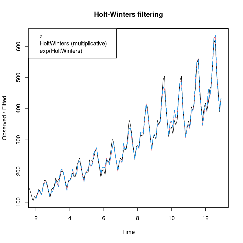
plot (m_smoothing_multi, lwd= 1 : 2 , lty= 1 : 2 )lines (exp (m_smoothing$ fitted[,1 ]), col= 4 , lty= 2 , lwd= 2 )legend ("topleft" , legend= c ("z" , "HoltWinters (multiplicative)" , "exp(HoltWinters)" ))
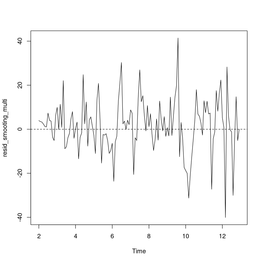
- 승법모형에 대한 잔차분석
<- resid (m_smoothing_multi)plot.ts (resid_smooting_multi)abline (h= 0 , lty= 2 )
예측오차의 경우 0을 중심으로 대칭이고, 이분산성은 없어 보인다.
t.test (resid_smooting_multi)
    One Sample t-test

data:  resid_smooting_multi
t = 1.5746, df = 131, p-value = 0.1178
alternative hypothesis: true mean is not equal to 0
95 percent confidence interval:
 -0.4315512  3.7983414
sample estimates:
mean of x
 1.683395
t-test 결과 예측오차의 평균은 0이라고 할 수 있다.
DW test 결과 예측오차들 간의 자기 상관이 있는 것으로 보인다.
하지만, 추세모형을 적합하였을 때 얻어진 잔차에 비해 유의확률값이 크지만, 가법 모형을 사용한 평활법에 비하면 조금 크다.
차이가 크지 않지만, 가법 모형이 더 적절하다고 할 수 있다. 따라서 가법 모형 사용.
(4)
로그변환한 데이터에 대한 가법모형을 사용하거나, 원래 데이터에 대한 승법 모형 적합 가능
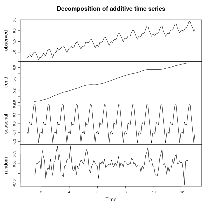
decompose 함수 사용
<- decompose (log_z_ts, 'additive' )plot (m_decompose_add)
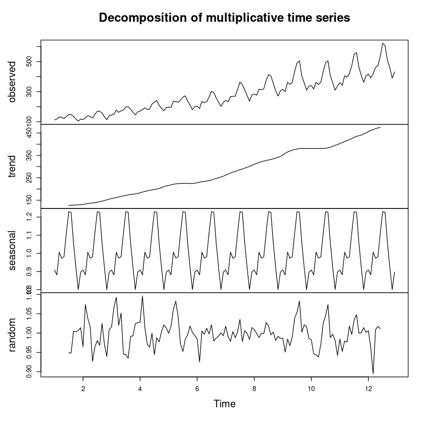
<- decompose (z_ts, 'multiplicative' )plot (m_decompose_multi)
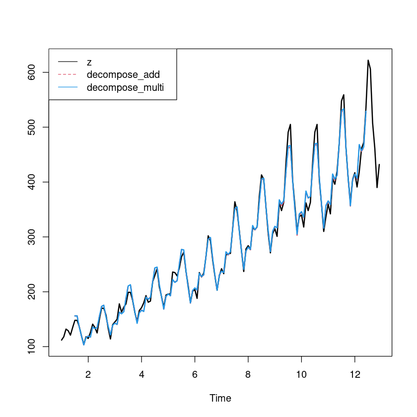
<- m_decompose_add$ trend + m_decompose_add$ seasonal #가법모형은 더 <- m_decompose_multi$ trend * m_decompose_multi$ seasonal #승법모
ts.plot (z_ts, exp (fitted_dec_add), fitted_dec_multi, col= c (1 ,2 ,4 ), lwd= 2 , lty= 1 : 2 )legend ("topleft" , c ("z" ,"decompose_add" , "decompose_multi" ), col= c (1 ,2 ,4 ), lty= 1 : 2 )
가법모형과 승법 모형은 차이가 거의 없어 보임
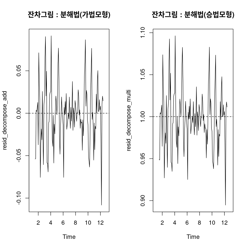
- 잔차분석을 하라는 문제는 없었지만 한 번 해보겠음.
<- m_decompose_add$ random<- m_decompose_multi$ randompar (mfrow= c (1 ,2 ))plot.ts (resid_decompose_add, main= "잔차그림 : 분해법(가법모형)" )abline (h= 0 , lty= 2 )plot.ts (resid_decompose_multi, main= "잔차그림 : 분해법(승법모형)" )abline (h= 1 , lty= 2 )
t.test (resid_decompose_add)t.test (resid_decompose_multi, mu= 1 )
    One Sample t-test

data:  resid_decompose_add
t = -0.28335, df = 131, p-value = 0.7774
alternative hypothesis: true mean is not equal to 0
95 percent confidence interval:
 -0.006909609  0.005178249
sample estimates:
  mean of x
-0.00086568
    One Sample t-test

data:  resid_decompose_multi
t = -0.59098, df = 131, p-value = 0.5556
alternative hypothesis: true mean is not equal to 1
95 percent confidence interval:
 0.992186 1.004219
sample estimates:
mean of x
0.9982026
t-test 결과 가법모형에서 예측오차의 평균은 0이라고 할 수 있고, 승법모형에서 예 측오차의 평균은 1이라고 할 수 있다
:: dwtest (lm (resid_decompose_add~ 1 ), alternative= "two.sided" ):: dwtest (lm (resid_decompose_multi~ 1 ), alternative= "two.sided" )
    Durbin-Watson test

data:  lm(resid_decompose_add ~ 1)
DW = 1.1441, p-value = 7.258e-07
alternative hypothesis: true autocorrelation is not 0
    Durbin-Watson test

data:  lm(resid_decompose_multi ~ 1)
DW = 1.1426, p-value = 6.946e-07
alternative hypothesis: true autocorrelation is not 0
DW test 결과 가법,승법 모두 예측오차들 간의 자기 상관이 있는 것으로 보인다.
(5)
주의 : 예측오차의 제곱합을 구하기 위해서는 로그변환한 자료를 사용한 분석 방법 의 경우 지수함수를 이용한 역변환을 한 후 계산해야 한다.
<- z- exp (fitted (m_trend)) #추세모형을 적합한 경우의 예측오차 <- z[- (1 : 12 )]- exp (m_smoothing$ fitted[,1 ]) #평활(가법)을 적합한 경 <- z[- (1 : 12 )]- m_smoothing_multi$ fitted[,1 ] #평활(가법)을 적합한 <- z - exp (fitted_dec_add) #분해법(가법)을 적합한 경우의 예측오차 <- z - fitted_dec_multi #분해법(승법)을 적합한 경우의 예측오차
#SSE <- sum (e_trend^ 2 , na.rm= T)<- sum (e_smoothing_add^ 2 , na.rm= T)<- sum (e_smoothing_multi^ 2 , na.rm= T)<- sum (e_decompose_add^ 2 , na.rm= T)<- sum (e_decompose_multi^ 2 , na.rm= T)
paste0 ("추세분석에서의 SSE = " , sse1)paste0 ("가법 계절평활법에 의한 SSE = " , sse2)paste0 ("승법 계절평활법에 의한 SSE = " , sse3)paste0 ("가법 분해법에 의한 SSE = " , sse4)paste0 ("승법 분해법에 의한 SSE = " , sse5)
'추세분석에서의 SSE = 49268.5277996137'
'가법 계절평활법에 의한 SSE = 20103.3932111226'
'승법 계절평활법에 의한 SSE = 20138.5987482274'
'가법 분해법에 의한 SSE = 15284.0239261845'
'승법 분해법에 의한 SSE = 14748.922939659'
#MSE <- mean (e_trend^ 2 , na.rm= T)<- mean (e_smoothing_add^ 2 , na.rm= T)<- mean (e_smoothing_multi^ 2 , na.rm= T)<- mean (e_decompose_add^ 2 , na.rm= T)<- mean (e_decompose_multi^ 2 , na.rm= T)
paste0 ("추세분석에서의 MSE = " , mse1)paste0 ("가법 계절평활법에 의한 MSE = " , mse2)paste0 ("승법 계절평활법에 의한 MSE = " , mse3)paste0 ("가법 분해법에 의한 MSE = " , mse4)paste0 ("승법 분해법에 의한 MSE = " , mse5)
'추세분석에서의 MSE = 342.142554163984'
'가법 계절평활법에 의한 MSE = 152.298433417596'
'승법 계절평활법에 의한 MSE = 152.565142032026'
'가법 분해법에 의한 MSE = 115.788060046852'
'승법 분해법에 의한 MSE = 111.734264694387'
MSE 역시 승법 분해법을 이용했을 때 가장 작은 값을 갖는다